A call detail record (CDR) is a data collected by telephone operators. It contains a sender, a receiver, a timestamp and the duration in case of a call. It is usually aggregated for customer’s privacy matter. The CDR we use for this analysis is a public dataset collected in the region of Milan in Italy. The dataset is available on Kaggle and called mobile phone activity. The CDR is pretty rich in information. The analysis in this post is based on the sms traffic. The data we use is then: the emitting antenna identifier, the receiving country and call counts. The goal of the analysis is to group antennas because their originating calls are similarly distributed over countries and - simultaneously - group countries because the received calls are distributed over the same antennas. This is called co-clustering. To do so, will first use a method based on information theory and define a set of measures to understand and visualize the results. Then, we will link the information theory to bayesian modeling, showing the benefits and difficulties using such an approach.

1. Data representation
2. Information theoretic coclustering
3. Bayesian blockmodeling
4. References

Data representation

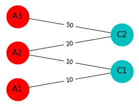
Let’s start by analyzing the data. The data set is a contingency table with the following columns: the emitting antenna, the receiving country and a decimal representing the number of calls for a certain area covered by an antenna. This number has been multiplied by a constant so that the real data cannot be reconstructed. In this post, we consider the data as a bipartite graph, i.e a graph containing two sets of nodes (the antennas and the countries). Edges connect one set to the other but cannot connect nodes belonging to the same set. Let’s consider a simple example. We have the following contingency table:

Antenna Id	Country Id	calls
A1	C1	10
A2	C1	10
A2	C2	20
A3	C2	50

Let’s turn this contigency table into a graph representation.

Bipartite graphs are also often represented as adjacency matrices: rows represent one set of nodes (for example the antennas) and the columns represent the other set of node (for example the countries). The cells of the matrix correspond to the interractions density between both set of nodes, in the running example, it is the number of calls from an antenna to a country. The adjacency matrix of the toy example above can be written as follows:

$$\begin{align} A = \begin{pmatrix} 10 & 0 \\ 10 & 20 \\ 0 & 50 \end{pmatrix} \end{align}$$

Information theoretic coclustering

Let’s define \(A\) the adjacency matrix of size \(n \times m\) (number of antennas \(\times\) number of countries) and \(C\) the partition of \(A\) into \(k \times l\) blocks (number of clusters of antennas \(\times\) number of clusters of countries). The matrix \(C\) is a compressed version of the matrix \(A\). Compression consists in reducing a large matrix to a smaller matrix, with the minimal information loss. To measure the information loss, we can use the so-called Kullback-Leibler divergence. This concept originates in information theory and measures how many bits we lose to encode a signal A from a signal B. In the present context, we can use it to compare two distributions. Let’s introduce \(P_A\), the joint probability matrix representing the adjacency matrix \(A\), i.e the matrix \(A\) that has been normalized by the total number of calls. Similarly, \(P_C\) is the joint probability matrix of the cluster adjacency matrix \(C\). Finally, \(\hat{P}_A\) is a joint probability matrix of size \(n \times m\) where cell values are the values of the joint probability between coclusters, normalized by the number of cells in the coclusters. Let’s illustrate it:

$\begin{align} A = \begin{pmatrix} 0 & 0 & 2 \\ 0 & 0 & 2 \\ 1 & 2 & 0 \\ 1 & 2 & 0 \end{pmatrix} & \Rightarrow & P_A = \begin{pmatrix} 0 & 0 & 0.2 \\ 0 & 0 & 0.2 \\ 0.1 & 0.2 & 0 \\ 0.1 & 0.2 & 0 \end{pmatrix} \end{align}$
$\begin{align} C = \begin{pmatrix} 0 & 4 \\ 6 & 0 \end{pmatrix} & \Rightarrow & P_C = \begin{pmatrix} 0 & 0.4 \\ 0.6 & 0 \end{pmatrix} & \Rightarrow & \hat{P}_A = \begin{pmatrix} 0 & 0 & 0.2 \\ 0 & 0 & 0.2 \\ 0.15 & 0.15 & 0 \\ 0.15 & 0.15 & 0 \end{pmatrix} \end{align}$

The Kullback-Leibler is a non symmetric measure and should be read as follow: \(KL(P_A \mid \hat{P}_A)\) denotes the Kullback-Leibler divergence from distribution \(\hat{P}_A\) to \(P_A\). This is defined as follows:

$$KL(P_A \mid \hat{P}_A) = P_A \log \left( \dfrac{P_A}{\hat{P}_A} \right)$$

Let’s illustrate the Kullback-Leibler divergence using a simple example. I need 3 apples, 2 oranges and 1 pear to bake a cake. Unfortunately, I can get from the supermarket only bags containing 1 apple, 1 orange and 1 pear. At the end, to make the cake, I need to buy 3 bags and there is 2 pears an 1 orange left. Lets turn is as distributions, the cakes contains 50% apples, 33% oranges and 17% pear. The bags from the supermarket contains 33% of each fruit. The Kullback-Leibler divergence from the bag distribution to the cake distribution is equal to 0.4. Let’s now analysis the edge cases: if both the bags and the cake have the same distribution, the Kullback Leibler divergence is null because the there is no fruit left after baking the cake. Conversly, if the bag does not contain oranges, the Kullback Leibler is infinite because, even with an infinite amount of bag, you are not going to bake the cake.

In information theoretic clustering, we try to find the optimal compressed matrix \(C\) which minimizes the Kullback-Leibler divergence to the joint probability distribution of the original adjacency matrix \(A\), i.e \(KL(P_A \mid \hat{P}_A)\). The Kullback Leibler divergence ranges in theory from \(0\) to \(+\infty\), but in the context of co-clustering, the latter case does not happen because there must be interractions between a cluster of antennas and a cluster of countries if the antennas (resp. the countries) it contains have interractions.

To optimize the Kullback-Leibler divergence, we use the following algorithm:

1. Initialize random clusters of antennas and countries
2. For each antenna, find the cluster minimizing the Kullback-Leibler divergence
3. For each country, find the cluster minimizing the Kullback-Leibler divergence
4. Update the clusters
5. Reiterate until clusters don’t change anymore.

The implementation is available on Github.

Let us analyze the results after running the algorithm with 5 clusters of countries and 6 clusters of antennas. We focus first on the clusters of country:

Cluster id	Countries (>1% overall traffic)
1	Senegal, Mali, Ivory Coast
2	Ukraine, Romania, Moldova
3	China, Philippines, Sri Lanka, Peru, Ecuador
4	Egypt, Bangladesh, Morocco, Pakistan
5	EU, Russia, USA

We can observe a pretty strong correlation between clusters of countries and regions of the world: the first cluster groups African countries, the second one Eastern European countries (except Russia), the third one groups South East Asia and South America, the fourth contains countries from North Africa to Asia through Middle East. Finally the fifth clusters corresponds to so-called western countries. Let’s now plot the clusters of antennas on a map.

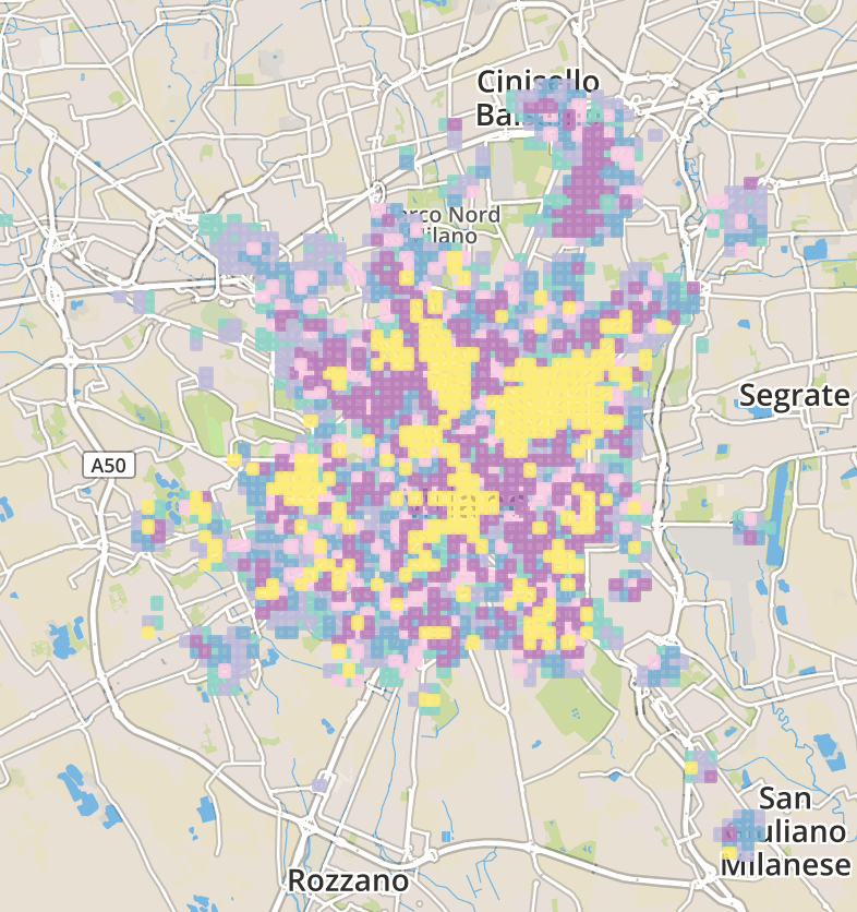
A zoomable map is available on Github. Clusters of antennas don’t show any obvious geographical correlation. The yellow cluster groups contiguous antennas, mainly located within Milan downtown. Also crimson antennas are mostly located in the city center. Other antennas are however spread in the outskirts of the city.

To understand the the clustering, we need to visualize interractions between clusters of countries and clusters of antennas. To that end, let’s introduce the concept of mutual information. Mutual information measures how much the partition of countries give information about the partition of antenna, and vice versa. In other words, it measure how confident we are guessing the originating antenna knowing the destination country of the call. Minimizing the Kullback-Leibler divergence is actually equivalent to minizing the loss in mutual information between the original data and the compressed data, that is exactly what the algorithm detailed above aims to do. The mutual information matrix is defined as follows:

$$MI_{ij}(P_C) = P_{C,ij} \log \left( \dfrac{P_{C,ij}}{P_{C,i} P_{C,j}} \right)$$

Let’s use a simple example to illustrate the behavior of the mutual information:

$$A = \begin{pmatrix} 0 & 0 & 2 & 1 \\ 0 & 0 & 2 & 1 \\ 1 & 2 & 0 & 0 \\ 1 & 2 & 0 & 0 \end{pmatrix}$$

Imagine we want to partition rows and columns into 2 clusters, i.e 4 blocks in the matrix. Grouping antennas 1 and 2, as well as antennas 3 and 4 produces the best partition. Indeed, both antennas 1 and 2 are linked to 3 and 4, and in the same proportions. Conversely, grouping 1 and 3, as well as 2 and 4 produces the worst partition. The best partition is called \(C_B\) and the worst partition \(C_W\) (with respective joint probability matrices \(P_B\) and \(P_W\)).

$$\begin{align} C_B = \begin{pmatrix} 0 & 6 \\ 6 & 0 \end{pmatrix} & \mbox{ } & C_W = \begin{pmatrix} 3 & 3 \\ 3 & 3 \end{pmatrix} \\\\ P_B = \begin{pmatrix} 0 & \frac{1}{2} \\ \frac{1}{2} & 0 \end{pmatrix} & \mbox{ } & P_W = \begin{pmatrix} \frac{1}{4} & \frac{1}{4} \\ \frac{1}{4} & \frac{1}{4} \end{pmatrix} \\\\ MI(P_B) = \begin{pmatrix} 0 & \frac{1}{2}\log(2) \\ \frac{1}{2}\log(2) & 0 \end{pmatrix} & \mbox{ } & MI(P_W) = \begin{pmatrix} 0 & 0 \\ 0 & 0 \end{pmatrix} \end{align}$$

The mutual information of the worst partition is null. In such a partition, occurences are distributed over the blocks and does not reflect the underlying structure of the initial matrix. This is the lowest bound of the mutual information. Conversely, the best partition maximizes the mutual information.

To evaluate the quality of the clustering, we visualise two matrices. First, the joint probability matrix \(P_C\). Second, the mutual information matrix \(MI(P_C)\).

First, let’s plot the two matrices for the randomly initialized clusters.

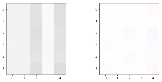
We can see on Figure 2 that the density is similarly distributed in the cell of the matrix. The mutual information also indicates that the density in the cells is close to the expected value in case of random clustering. In other words, \(P_{C,ij} \simeq P_{C,i} P_{C,j}\). Once Kullback-Leibler divergence has been maximized, we can observe the underlying structure of the data emerging.

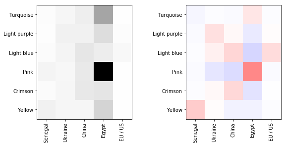
On Figure 3, the joint probability shows cells with high density. But this observation does not mean that the partition is meaningful. In the mutual information matrix, red cells represent excess of cooccurrences. Conversely, blue cells respresent lacks of cooccurences. The clusters can then be interpreted as follow: antennas in pink are grouped together because there is an more calls than expeted to Egypt but less than expected to China and Ukraine. Note that there is a high amount of calls from antennas in yellow to Egypt, however less than expected in case of independence.

Bayesian blockmodeling

Information theoretic clustering directly optimizes the Kullback-Leibler divergence from the partition to the actual data. This approach is valid when the amount of data is large enough to properly estimate the joint probability matrix between antennas and countries. But if it’s not the case, we can easily get spurious patterns. One solution to avoid this problem consists in adding a regulariuation term to the optimized criterion. Another solution would be to build a Bayesian model. Actually, the average negative logarithm of the multinomial probability mass function over the cells of the adjacency matrix converges to the Kullback-Leibler divergence from the partition to the actual data.

$$KL(P_A | \hat{P}_A) \rightarrow -\dfrac{1}{n} \log(f_\mathcal{M}(n, A, \hat{P}_A)) \mbox{ when } n \rightarrow +\infty$$

where n is the number of observations (sms in th example) and \(f_\mathcal{M}\) the probability mass function of the multinomial distribution. This can be easily proved using the Stirling approximation, i.e \(\log(n!) \rightarrow n\log(n) - n\) ; when \(n \rightarrow +\infty\).

References

Inderjit S. Dhillon et al., Information-theoretic co-clustering, KDD 2003