
Tutorial - How to evaluate the confidence in a percentage?
Percentage is one of the most common mathematical concept. At this time of world cup, a poll has been conducted to evaluate the football enthusiasm of the population of France. It appeared that 64% of surveyed people declared planning to watch the games and they were right (edit July 15th, 2018). This percentage has a confidence attached to it. The bigger the confidence, the more accurate the percentage and the more it can be generalized to the overall population. This confidence is seldom mentioned in the news. The goal of this tutorial is to show how to assess whether a percentage or a probability has been correctly estimated and how big the confidence interval is. Let’s use the example of the poll on football as an illustration.
Note: this is the blog version of the tutorial. If you want to reproduce the experiments, you can check the corresponding Jupyter Notebook.

Definition
The percentage of people planning to watch the football games is defined as the number of people planning to watch the games divided by the number of surveyed people.
Problem
What if only 10 persons would have been surveyed? Would you feel confident generalizing to the rest of the population of the country? To answer that question, several statistical tools can be used.
Bootstrapping
Definition
Bootstrapping consists in randomly sampling observations with replacement, that is, every person is surveyed independently from another and the probability of getting a certain answer does not affect the probability of the answers of the next surveyed persons.
Illustration
Imagine 10 persons are in a room and 10 interviewers are waiting outside the room. The first interviewer enters the room, asks one person whether she plans to watch the games, and leaves the room. Then, the second interviewer repeats the same process without knowing who has answered the previous interviewer. And so on for the next 8 interviewers.
Once all ten interviewers have collected an answer, we can compute the percentage of interviewers who got a “yes”.
Question: is this percentage accurate?
No. To see it, we can repeat the full process several times and check the obtained results. Let’s do it 3 times:
50.0% of surveyed persons plan to watch the games.
60.0% of surveyed persons plan to watch the games.
We can observe that for a sample of only 10 persons, the percentage varies a lot. The challenge is to find out how many persons we need to survey to get a reliable percentage estimation.
Let’s repeat the experience 1,000 times for different sample sizes. On the Figure below, x axis is the number of surveyed persons (log scale), y axis is the percentage of people declaring they plan to watch the games, and the dots corresponds to the obtained result for each of the 1,000 trials.
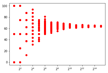
The figure above shows that the more we survey people, the more the percentage we obtain converge to 64.0%.
Question how can we assess the confidence in the estimation of a calculated percentage?
One option consists in computing the average percentage and the standard deviation for each number of surveyed persons. In the following plot, bars are twice the standard deviation, so that we get confidence intervals at a 95% precision level.
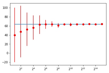
For 4 surveyed persons, the percentage of persons watching the games is 47.5 (± 56.8)%
For 8 surveyed persons, the percentage of persons watching the games is 52.5 (± 36.7)%
For 16 surveyed persons, the percentage of persons watching the games is 56.3 (± 26.8)%
For 32 surveyed persons, the percentage of persons watching the games is 62.8 (± 20.6)%
For 64 surveyed persons, the percentage of persons watching the games is 63.4 (± 9.6)%
For 128 surveyed persons, the percentage of persons watching the games is 64.0 (± 6.0)%
For 256 surveyed persons, the percentage of persons watching the games is 61.1 (± 4.9)%
For 512 surveyed persons, the percentage of persons watching the games is 63.5 (± 2.2)%
The binomial confidence interval
Bootstrapping is simple and intuitive but sampling is a pretty heavy process for evaluating a percentage.
Question: Is there a way to compute directly the confidence using the numbers of surveyed persons and the calculated percentage?
Of course, there is! This is called the binomial estimator.
The binomial estimator considers the problem the opposite way: how likely it is that the results of the survey are sampled from the percentage. Concretely, we know that 64% of french people plan to watch the games, how likely is it that in a sample of 100 persons, 64 of them are going to watch the football games?
For 10,000 surveyed persons, the probability that 6,400 of them plan to watch the game, if the expected percentage is 64%, is equal to 0.83%
This is quite counterintuitive: the more there are observations, the less it is reliable. But it is also more likely to find randomly 64 persons planning to watch the games over 100 surveyed people than 6,400 over 10,000.
The probability to randomly find 6,400 persons planning to watch the games over 10,000 surveyed people is 0.01%.
Question: How to derive the confidence interval from it?
Let’s do some maths! Let’s write the binomial estimator as a conditional probability: \(P(k \mid n, p)\).
Example: In the survey published in the news, 1,000 persons were surveyed. Then, \(P(k=640 \mid n=1000, p=0.64)\) denotes the probability to find 640 persons planning to watch the games over 1,000 surveyed people knowing that the expected percentage is 64%.
Let’s suppose that we want a confidence interval at a 95% precision level. To obtain it, we must find the lower (610) and the upper (670) interval, so that 95% of the area under the binomial density curve is located within an interval centered around the expected number (640) of persons planning watching the games. The figure below illustrates the confidence interval.
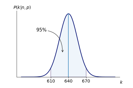
Conclusion: For 1,000 surveyed persons, if we find 640 persons planning to watch the games, then the percentage is equal to 64 (± 3)%, at a 95% precision level.
Question: Is there a way to compute it directly?
Yes. There is also a way to estimate that value:
where \(p\) is the percentage, \(n\) is the number of samples and z is the z value, constant value depending on the required precision. The z value is pretty difficult to compute. Here is a table for common precision values:
| Precision | Error rate | Z value |
|---|---|---|
| 68.2% | 31.8% | 1.00 |
| 90.0% | 10.0% | 1.64 |
| 95.0% | 5.0% | 1.96 |
| 99.0% | 1.0% | 2.58 |
Now let’s plot the same chart as we did for bootstrapping. And note that we obtain similar confidence intervals.
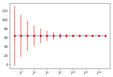
For 4 surveyed persons, the percentage of persons watching the games is 64.0 (± 47.0)%
For 8 surveyed persons, the percentage of persons watching the games is 64.0 (± 33.3)%
For 16 surveyed persons, the percentage of persons watching the games is 64.0 (± 23.5)%
For 32 surveyed persons, the percentage of persons watching the games is 64.0 (± 16.6)%
For 64 surveyed persons, the percentage of persons watching the games is 64.0 (± 11.8)%
For 128 surveyed persons, the percentage of persons watching the games is 64.0 (± 8.3)%
For 256 surveyed persons, the percentage of persons watching the games is 64.0 (± 5.9)%
For 512 surveyed persons, the percentage of persons watching the games is 64.0 (± 4.2)%
Comparing two proportions
Imagine we want to compare the evolution of a percentage month over month. Let’s use another example here. The news claim that satisfaction rate of citizens with the actions lead by the president dropped from 45% to 43%. A survey has been conducted on a sample of 1,000 persons.
Question: How can we assess whether this change is relevant or not?
First, we can have a look at the confidence intervals of the two percentage, at a 95% precision level.
The satisfaction rate in June is 43.0 (±3.0)%
In this case, we observe a decrease of 2pp of the satisfaction rate between May and June. The confidence intervals overlap but this is not enough to draw any conclusion.
Question: Can we directly compute a confidence interval on the decrease itself?
Yes, in a similar way to how we did it for computing the confidence interval of a percentage:
where \(p_1\) and \(p_2\) are the percentages and \(n_1\) and \(n_2\) the number of surveyed persons, of respectively the first and the second month.
Conclusion: The confidence interval is higher than the evolution itself. This means that the sample size of the surveyed population is too small to conclude from the confidence interval of an evidence of a decrease, that can be generalized to the entire population of the country. This analysis does not however question the fact that there is a trend of decrease. To make the number statistically more relevent, a solution would be to increase the number of surveyed people. Another solution would be to aggregate the numbers on a longer time period, for example on a quarter (3 months). In that case, the confidance interval would decrease to 2.5pp with a 95% precision.