
Tutorial - Word2vec using pytorch
This notebook introduces how to implement the NLP technique, so-called word2vec, using Pytorch. The main goal of word2vec is to build a word embedding, i.e a latent and semantic free representation of words in a continuous space. To do so, this approach exploits a shallow neural network with 2 layers. This tutorial explains:
- how to generate the dataset suited for word2vec
- how to build the neural network
- how to speed up the approach
The data
Let’s introduce the basic NLP concepts:
- Corpus: the corpus is the collection of texts that define the data set
- vocabulary: the set of words in the data set.
For the example, we use the news corpus from the Brown dataset, available on nltk. Non letter characters are removed from the string. Also the text is set in lowercase.
import re
import nltk
nltk.download('brown')
from nltk.corpus import brown

corpus = []

for cat in ['news']:
    for text_id in brown.fileids(cat):
        raw_text = list(itertools.chain.from_iterable(brown.sents(text_id)))
        text = ' '.join(raw_text)
        text = text.lower()
        text.replace('\n', ' ')
        text = re.sub('[^a-z ]+', '', text)
        corpus.append([w for w in text.split() if w != ''])
Subsampling frequent words
The first step in data preprocessing consists in balancing the word occurences in the data. To do so, we perform subsampling of frequent words. Let’s call \(p_i\) the proportion of word \(i\) in the corpus. Then the probability \(P(w_i)\) of keeping the word in the corpus is defined as follows:
from collections import Counter
import random, math

def subsample_frequent_words(corpus):
    filtered_corpus = []
    word_counts = dict(Counter(list(itertools.chain.from_iterable(corpus))))
    sum_word_counts = sum(list(word_counts.values()))
    word_counts = {word: word_counts[word]/float(sum_word_counts) for word in word_counts}
    for text in corpus:
        filtered_corpus.append([])
        for word in text:
            if random.random() < (1+math.sqrt(word_counts[word] * 1e3)) * 1e-3 / float(word_counts[word]):
                filtered_corpus[-1].append(word)
    return filtered_corpus
corpus = subsample_frequent_words(corpus)
vocabulary = set(itertools.chain.from_iterable(corpus))

word_to_index = {w: idx for (idx, w) in enumerate(vocabulary)}
index_to_word = {idx: w for (idx, w) in enumerate(vocabulary)}
Building bag of words
Word2vec is a bag of words approach. For each word of the data set, we need to extract the context words, i.e the neighboring words in a certain window of fixed length. For example, in the following sentence:
My cat is lazy, it sleeps all day long
If we consider the target word lazy, and chose window of size 2, then context words are cat, is, it and sleeps.
import numpy as np

context_tuple_list = []
w = 4

for text in corpus:
    for i, word in enumerate(text):
        first_context_word_index = max(0,i-w)
        last_context_word_index = min(i+w, len(text))
        for j in range(first_context_word_index, last_context_word_index):
            if i!=j:
                context_tuple_list.append((word, text[j]))
print("There are {} pairs of target and context words".format(len(context_tuple_list)))
The network
There two approach of word2vec:
- CBOW (Continuous Bag Of Words). It predicts the target word conditionally to the context. In other words, context words are the input and the target word is the output.
- Skip-gram. It predicts the context conditionally to the target word. In other words, the target word is the input and context words are the output.
The following code is suited for CBOW.
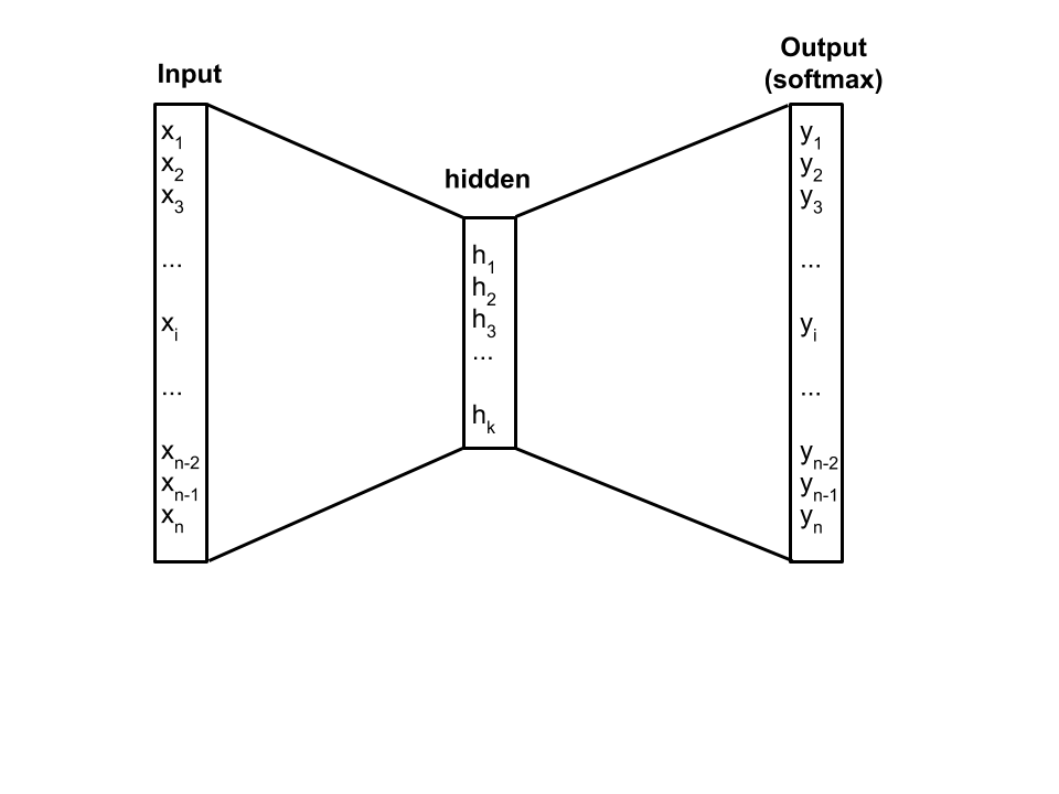
The vocabulary is represented as a one-hot encoding, meaning that the input variable is a vector of the size of the vocabulary. For a word, this vector has 0 at every position besides the word index in the vocabulary, where value is 1. The hot encoding is mapped to an embedding, i.e a latent representation of the word as a vector containing continuous values and which size is smaller than the one-hot encoding vector.
For each context word, a softmax function takes the embedding of the word, yielding a probability distribution of the target word over the vocabulary.
import torch
import torch.nntorch.nn  as  nn
import torch.autogradtorch.aut  as autograd
import torch.optim as optim
import torch.nn.functional as F


class Word2Vec(nn.Module):

    def __init__(self, embedding_size, vocab_size):
        super(Word2Vec, self).__init__()
        self.embeddings = nn.Embedding(vocab_size, embedding_size)
        self.linear = nn.Linear(embedding_size, vocab_size)

    def forward(self, context_word):
        emb = self.embeddings(context_word)
        hidden = self.linear(emb)
        out = F.log_softmax(hidden)
        return out
Early stopping
Before starting learning, let’s introduce the concept of early stopping. It aims at stopping learning when the loss does not decrease significantly (min_percent_gain parameter) anymore after a certain number of iterations (patience parameter). Early stopping is usually used on the validation loss, but in the case of word2vec, there is no validation since the approach is unsupervised. We apply early stopping on training loss instead.
class EarlyStopping():
    def __init__(self, patience=5, min_percent_gain=0.1):
        self.patience = patience
        self.loss_list = []
        self.min_percent_gain = min_percent_gain / 100.

    def update_loss(self, loss):
        self.loss_list.append(loss)
        if len(self.loss_list) > self.patience:
            del self.loss_list[0]

    def stop_training(self):
        if len(self.loss_list) == 1:
            return False
        gain = (max(self.loss_list) - min(self.loss_list)) / max(self.loss_list)
        print("Loss gain: {}%".format(round(100*gain,2)))
        if gain < self.min_percent_gain:
            return True
        else:
            return False
Learning
For learning, we use cross entropy as a loss function. The neural network in trained with the following parameters:
- embedding size: 200
- batch size: 2000
vocabulary_size = len(vocabulary)

net = Word2Vec(embedding_size=2, vocab_size=vocabulary_size)
loss_function = nn.CrossEntropyLoss()
optimizer = optim.Adam(net.parameters())
early_stopping = EarlyStopping()
context_tensor_list = []

for target, context in context_tuple_list:
    target_tensor = autograd.Variable(torch.LongTensor([word_to_index[target]]))
    context_tensor = autograd.Variable(torch.LongTensor([word_to_index[context]]))
    context_tensor_list.append((target_tensor, context_tensor))

while True:
    losses = []
    for target_tensor, context_tensor in context_tensor_list:
        net.zero_grad()
        log_probs = net(context_tensor)
        loss = loss_function(log_probs, target_tensor)
        loss.backward()
        optimizer.step()
        losses.append(loss.data)
    print("Loss: ", np.mean(losses))
    early_stopping.update_loss(np.mean(losses))
    if early_stopping.stop_training():
        break
Speed up the approach
The implementation introduced is pretty slow. But good news, there are solutions for speeding up the computation.
Batch learning
In order to speed up the learning, we propose to use batches. This implies that a bunch of observations are forwarded through the network before doing the backpropagation. Besides being faster, this is also a good way to regularize the parameters of the model.
import random

def get_batches(context_tuple_list, batch_size=100):
    random.shuffle(context_tuple_list)
    batches = []
    batch_target, batch_context, batch_negative = [], [], []
    for i in range(len(context_tuple_list)):
        batch_target.append(word_to_index[context_tuple_list[i][0]])
        batch_context.append(word_to_index[context_tuple_list[i][1]])
        batch_negative.append([word_to_index[w] for w in context_tuple_list[i][2]])
        if (i+1) % batch_size == 0 or i == len(context_tuple_list)-1:
            tensor_target = autograd.Variable(torch.from_numpy(np.array(batch_target)).long())
            tensor_context = autograd.Variable(torch.from_numpy(np.array(batch_context)).long())
            tensor_negative = autograd.Variable(torch.from_numpy(np.array(batch_negative)).long())
            batches.append((tensor_target, tensor_context, tensor_negative))
            batch_target, batch_context, batch_negative = [], [], []
    return batches
Negative examples
The default word2vec algorithm exploits only positive examples and the output function is a softmax. However, using a softmax slows down the learning: softmax is normalized over all the vocabulary, then all the weights of the network are updated at each iteration. Consequently we decide using a sigmoid function as an output instead: only the weights involving the target word are updated. But then the network does not learn from negative examples anymore. That’s why we need to input artificially generated negative examples.
Once we have built the data for the positive examples, i.e the words in the neighborhood of the target word, we need to build a data set with negative examples. For each word in the corpus, the probability of sampling a negative context word is defined as follows:
from numpy.random import multinomial

def sample_negative(sample_size):
    sample_probability = {}
    word_counts = dict(Counter(list(itertools.chain.from_iterable(corpus))))
    normalizing_factor = sum([v**0.75 for v in word_counts.values()])
    for word in word_counts:
        sample_probability[word] = word_counts[word]**0.75 / normalizing_factor
    words = np.array(list(word_counts.keys()))
    while True:
        word_list = []
        sampled_index = np.array(multinomial(sample_size, list(sample_probability.values())))
        for index, count in enumerate(sampled_index):
            for _ in range(count):
                 word_list.append(words[index])
        yield word_list
import numpy as np

context_tuple_list = []
w = 4
negative_samples = sample_negative(8)

for text in corpus:
    for i, word in enumerate(text):
        first_context_word_index = max(0,i-w)
        last_context_word_index = min(i+w, len(text))
        for j in range(first_context_word_index, last_context_word_index):
            if i!=j:
                context_tuple_list.append((word, text[j], next(negative_samples)))
print("There are {} pairs of target and context words".format(len(context_tuple_list)))
The network
The main difference from the network introduced above lies in the fact that we don’t need a probability distribution over words as an output anymore. We can instead have a probability for each word. To get that, we can replace the softmax out output by a sigmoid, taking values between 0 and 1.
The other main difference is that the loss needs to be computed on the observe output only, since we provide the expected output as well as a set of negative examples. To do so, we can use a negative logarithm of the output as a loss function.
For a target word \(w_T\), a context word \(w_C\) and a negative example \(w_N\), respective embeddings are defined as \(e_T\), \(e_C\) and \(e_N\). The loss function \(l\) is defined as follows:
import torch
import torch.nn as nn
import torch.autograd as autograd
import torch.optim as optim
import torch.nn.functional as F


class Word2Vec(nn.Module):

    def __init__(self, embedding_size, vocab_size):
        super(Word2Vec, self).__init__()
        self.embeddings_target = nn.Embedding(vocab_size, embedding_size)
        self.embeddings_context = nn.Embedding(vocab_size, embedding_size)

    def forward(self, target_word, context_word, negative_example):
        emb_target = self.embeddings_target(target_word)
        emb_context = self.embeddings_context(context_word)
        emb_product = torch.mul(emb_target, emb_context)
        emb_product = torch.sum(emb_product, dim=1)
        out = torch.sum(F.logsigmoid(emb_product))
        emb_negative = self.embeddings_context(negative_example)
        emb_product = torch.bmm(emb_negative, emb_target.unsqueeze(2))
        emb_product = torch.sum(emb_product, dim=1)
        out += torch.sum(F.logsigmoid(-emb_product))
        return -out
The neural network in trained with the following parameters:
- embedding size: 200
- batch size: 2000
import time

vocabulary_size = len(vocabulary)

loss_function = nn.CrossEntropyLoss()
net = Word2Vec(embedding_size=200, vocab_size=vocabulary_size)
optimizer = optim.Adam(net.parameters())
early_stopping = EarlyStopping(patience=5, min_percent_gain=1)

while True:
    losses = []
    context_tuple_batches = get_batches(context_tuple_list, batch_size=2000)
    for i in range(len(context_tuple_batches)):
        net.zero_grad()
        target_tensor, context_tensor, negative_tensor = context_tuple_batches[i]
        loss = net(target_tensor, context_tensor, negative_tensor)
        loss.backward()
        optimizer.step()
        losses.append(loss.data)
    print("Loss: ", np.mean(losses))
    early_stopping.update_loss(np.mean(losses))
    if early_stopping.stop_training():
        break
Once the network trained, we can use the word embedding and compute the similarity between words. The following function computes the top n closest words for a given word. The similarity used is the cosine.
import numpy as np

def get_closest_word(word, topn=5):
    word_distance = []
    emb = net.embeddings_target
    pdist = nn.PairwiseDistance()
    i = word_to_index[word]
    lookup_tensor_i = torch.tensor([i], dtype=torch.long)
    v_i = emb(lookup_tensor_i)
    for j in range(len(vocabulary)):
        if j != i:
            lookup_tensor_j = torch.tensor([j], dtype=torch.long)
            v_j = emb(lookup_tensor_j)
            word_distance.append((index_to_word[j], float(pdist(v_i, v_j))))
    word_distance.sort(key=lambda x: x[1])
    return word_distance[:topn]